Brief Notes on Neubig's Tutorial 0~3: Part A

1. Tutorial 0 - Setting up your environment and basic python

• The goal of this course:
  • During tutorial: learn something new: new concepts, new models, new algorithms etc.
  • And our adapted goal is: run the program during the tutorial, and let all the members watch and see the results.
  • Another encourage from Neubig is to work in pairs or small groups, this enables discussion and cooperation which will make every one within the group to learn 2 or 3 times efficiently and more.
• Programming language is not restricted to Python. However, I would really recommend Python as your quick working language or prototype language with which you can quickly develop some raw idea upon. Another reason is that python is so hot recently because of most of the deep learning framework supported python.

Setting up environment

It is very important for one to get familiar with his/her most suitable development environment. During this section Neubig gives some specific advice which I would like to add my owns.

• Be able to access to Google! This is very important since every time you want to look up something, maybe a command line or just some bug information prompted from you runtime python program. Just type/copy it in the Google search textarea. This will open a window of independence for yourself.

• Be familiar with linux terminal environment. In the future, most of your jobs will be working with Linux, typing ls /usr/local/cuda , cd ~/Workspace/Experiment ipython, mkdir, mv etc.

  • Login to a Linux machine. If you have a server id, like me, I have an account on 117 server which is on the LAN of our lab, you can log in on that machine via ssh glli@10.10.255.117(this is my log in command). Then you will be required for your password. But I would recommend using a linux client named MobaXterm which is an integrated client app that can hold a file management GUI and a terminal window, like the following. Since we call a connection between your local machine and the linux server as a session, you can manage your sessions through within the same Tab view, like tab management in Chrome and other browser.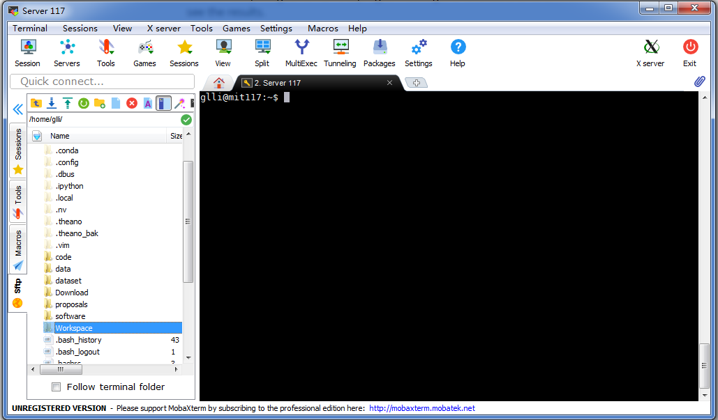

    

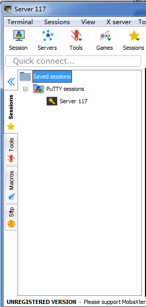
  • Create a session. The way to create a session is very simple, just click Session button in the tool bar, the first button along that row. And choose ssh connection and then type your Remote host IP and your username in Specify username. Then you can click OK to go on opening a terminal and input your password to log in. Note that: this session will saved and you can find it at the session tab at the left edge of your window with a star logo! You won’t miss it! Every time you want to create a new terminal, just double click your session. You can rename the session as I do in the following.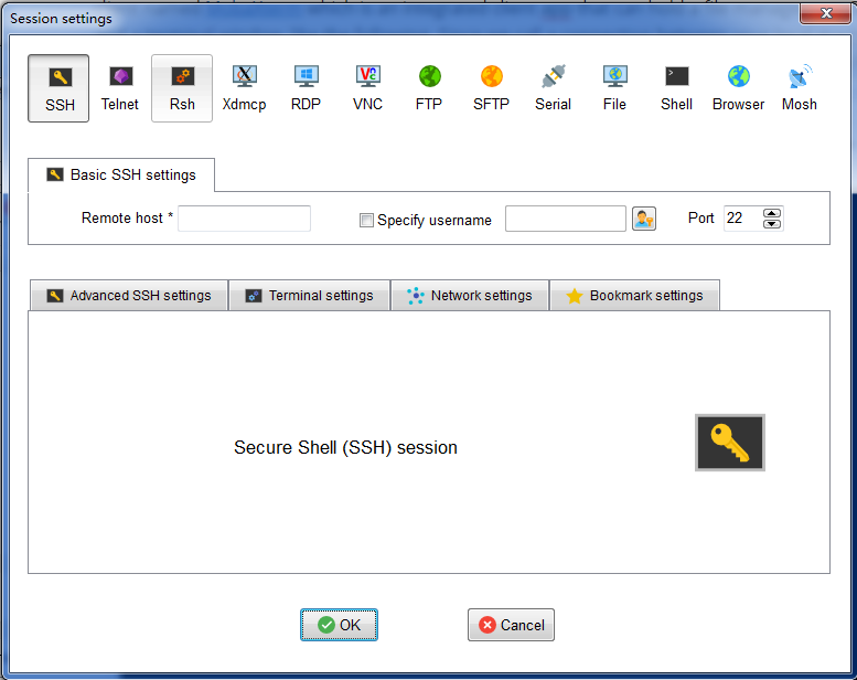

    

    

  • Use your favorite text editor. I recommend Sublime Text if you are not familiar with vim/gvim etc. Then your coding workflow will be like this: a). Open a source file through the sftp tab of MobaXterm using sublime; 2). Edit it, and save it using ctrl+s; 3). Debug it in the terminal, and go back to a). until you finish your work.

• Use git to clone the repo. Firstly, if you don’t have a github account please sign up one! (This does not bother you use git, a local app on your local machine or server, sign up one just because github is awesome.) In your local machine or server, cygwin or terminal, type git clone https://github.com/Epsilon-Lee/nlptutorial.git to get a local repo of the tutorial. If you are a fresh man on using git, try to learn more about it. I started this summer from here at Code academy.

Python basics

• Python data types. str, int and float etc. those are basic data types. You can use print("%s %f %d" % ('nlp', .3, 1)) where %s to hold string, %f to hold float and %d to hold integer.
• Python condition statement. if ... elif ... else ....
• Python advanced built-in data structure. list and dict. Know how to create, access, assign value to, delete value from, traverse, sort these two data structures. Try to use google to find every operations listed before.
• Python collection module. There are many great and useful sub-modules in the collection module, you can refer to this Chinese post for more knowledge.
• Python read text file, split line, count vocabulary. It is very common for researchers in NLP to create vocabulary from raw text files when working on a new task or project, so basic text file manipulation with python is essential for everyone.
• Unit test. Since I am not a software engineer and have not contribute to something sophisticated, I just don’t know the importance of doing unit test. But after I have some experience with a little bigger programs in Machine Learning, for example, a sequence-to-sequence attentional model for neural machine translation. It suddenly become necessary for me to modularize my project and test each modules with input-output guarantee! Otherwise, if I just run them as a whole, it would be hard for me to debug since I cannot remember every detail of the whole of my code.

2. Tutorial 1 - Language model basics

Why language models?

In this subsection, I would like to discuss more about language models. I mainly concern about the following questions:

1. What is a (probabilistic) model in practice and philosophically?
2. What is a parameterization of a model?
3. What is estimation of certain parameterization of a model?

This is a small question in terms of Neubig’s slides content. However, he is just try to use some example that could make sense to beginners for introducing the language models based on its utility aspect, that is, language models could score the output of a speech recognition system and help the system to response to its user the most natural (fluent, acceptable) recognized result. Of course, after making a little bit sense of the practical aspect of a language model, it is more valuable to know that language model is more than that!

To answer what is a language model philosophically, we should understand what is a model in a probabilistic point of view. Probabilistic model or model is a probability distribution, denoted as \(\mathbb{P} (\cdot)\), over certain sample space that we care most, so the distribution could be used to summarize statistical regularities and properties of the elements in the sample space. Intuitively, we call those elements as a kind of phenomenon from nature and human society. The usage of a model is to open our statistical toolkit for us human to describe phenomenon (you can call phenomenon data), to understand some statistical or even causal aspect of the phenomenon, or even to predict the occurrence of certain phenomenon of interest.

To have a direct feeling of language model, I refer you to the Google’s research blog All our n-gram are belong to you and this sample entries from www.ngram.info. You can see that, language models are just word sequence frequency.

Language model is used for human to summarize statistical/descriptive properties in language data! It is a probabilistic distribution over natural language, i.e. words, sentences, paragraphs etc.

Specifically speaking, we can use a language model to compute probability of a word sequence \(w_1, \dots, w_n\) if the minimum element of a language is word (this is not always true, since in Chinese or Japanese we can have characters which is subpart of a word.) We can get the symbolic representation as:

\[P(w_1, \dots, w_n)\]

There are many ways to parameterize the above probability formula.

Concept of parameterization. Parameterization is a very important and practical concepts in probabilistic modeling methods. The meaning of parameterization is: a kind of representation of the computational aspect of the model. More specifically that is given an element in the sample space, e.g. here we get a word sequence \(w_1, \dots, w_n\), we can use the parameterization as a way for calculating its probability. [A little bit abstract? Don’t worry, go on reading and re-think about the statement here.]

Another important aspect of parameterization is that this concept is usually used for [parametric models](https://en.wikipedia.org/wiki/Parametric_model) which is a probabilistic model that has some finite dimension of parameters whose values are determined/learned from data, i.e. fitting the model to the data or training the model, aka. machine learning! Intuitively speaking, if a model is a family of a certain descriptive method for the data, a specific parameter setting (that is a certain value of its parameters) decide a certain model in that family which has knowledge about its learning resource – the data. So the knowledge from data is “memorized” in those parameters!

One way to parameterize \(P(w_1, \dots, w_n)\) is to use the so-called bi-gram language model, which is depend on the 1st order Markov assumption as following. Since we can use probability chain rule to decompose \(P(w_1, \dots, w_n)\) as:

\[P(w_1, \dots, w_n) = P(w_1) P(w_2 \vert w_1) P(w_3 \vert w_1, w_2) \dots P(w_n \vert w_1 \dots w_{n-1})\]

Since probability chain rule is a theorem, the above equality holds strictly. Then according to the 1st order Markov assumption, we get that: \(P(w_i \vert w_{1:i-1}) = P(w_i \vert w_{i-1})\).

Probability Chain Rule. This rule is very important in probabilistic machine learning literature. It states that any joint probability could be decomposed into product of conditional probabilities. It is easy to write the above equality in a recursive manner for freshman to get familiar of the working of chain rule. That is you first decompose \(w_1,\dots,w_n\) it into: \(P(w_1) \cdot P(w_2,\dots,w_n \vert w_1)\), and then go on to decompose \(w_2,\dots,w_n\) into \(P(w_2 \vert w_1) \cdot P(w_3,\dots,w_n \vert w_1, w_2)\) and then go on this process recursively.

k-th order Markov Assumption. The Markov assumption means that the conditional probability of the current state \(s_t\) is independent with the history states if given its k previous states \(s_{i-k}, \dots, s_{i-1}\).

So for a bi-gram language model, we can get:

\[P(w_1, \dots, w_n) = P(w_1 \vert \cdot) P(w_2 \vert w_1) P(w_3 \vert w_2) \dots P(w_n \vert w_{n-1})\]

On the right hand side (RHS) of the above formula, it is very regular that each probability term has two specific symbols \(P( symbol_1 \vert symbol_2)\) with the conditional mark \(\vert\) in between. Note that, here the first term of the RHS used to \(P(w_1)\), but now we want to every term to be of the same form, we re-denote it as \(P(w_1 \vert \cdot)\), where the \(\cdot\) is a null symbol, or you can think of it as a beginning symbol denoting a sequence is beginning!

Bi-gram model. Note that we call this decomposition \(P(symbol_1 \vert symbol_2)\) bi-gram model, because we only consider the dependency between 2 adjacent words. So tri-gram model considers this \(P(symbol_1 \vert symbol_2, symbol_3)\) kind of dependency. And you can generalize to any n-gram models now.

The 2-gram or bi-gram language model is parameterized by a group of conditional probability terms with the above mentioned form. The parameters of this model are each conditional probability terms \(P(\cdot \vert \cdot)\) which has its value between \((0,1)\), but more constraints should be satisfied, see discussion below. If this term is with respect to word \(w_i\) and \(w_j\) with i after j, we denote it to look more like a parameter as \(\theta_{w_i \vert w_j}\). If we have a vocabulary of 10000, we will have about \(10000^2\) number of such terms (easy combinatorial math! Right?) as our model’s parameters. So if we have an accurate estimation of these parameters. We can use them and the decomposed formula to compute the probability of a sentence! For example, a sentence “I love my parents !” We can compute its probability according to our model or our model’s parameterization as following:

\[\begin{align} P(\text{"I love my parents !"}) &= P(\text{"<s> I love my parents ! </s>"}) \\ &= P(\text{"<s>"}) P(\text{"I"} \vert \text{"<s>"}) P(\text{"love"} \vert \text{"I"}) P(\text{"my"} \vert \text{"love"}) P(\text{"parents"} \vert \text{"my"}) P(\text{"!"} \vert \text{"parents"}) P(\text{"</s>"} \vert \text{"!"}) \\ &= \theta_{\text{"<s>"}} \theta_{\text{"I"} \vert \text{"<s>"}} \theta_{\text{"love"} \vert \text{"I"}} \theta_{\text{"my"} \vert \text{"love"}} \theta_{\text{"parents"} \vert \text{"my"}} \theta_{\text{"!"} \vert \text{"parents"}} \theta_{\text{"</s>"} \vert \text{"!"}} \end{align}\]

Here is a trick or taste! That is we augment the original word sequence with a start symbol \(\text{<s>}\) and an end symbol \(\text{</s>}\). So we can make every word in vocabulary to appear both at the left-hand and right-hand side of the conditional mark \(\vert\) which is a taste of statistical completeness. And since every word sequence will definitely start with a \(\text{<s>}\) symbol, so we know that \(P("\text{<s>}") = 1\).

Statistical estimation. Statistical estimation is to estimate the possible value or distribution of the model parameters. Their are many different flavors of statistical estimation. The main two categories are point estimation and interval estimation (a specific form of distribution estimation). a). Point estimation like maximum likelihood estimation (MLE), maximum posterior estimation (MAP) or Bayesian estimation by which the final estimation of the parameters is a point (just one specific value) in the parameter’s space. (Parameter space is a high-dimensional space \(\mathbb{R}^d\), if we have \(d\) parameters in our model.) Each of the methods of point estimation bears certain statistical advantage. b). Interval estimation or distribution estimation is to maintain a distribution which we call posterior in Bayesian statistics over the parameter space \(\mathbb{R}^d\). Intuitively speaking, a distribution has all the benefits over point distribution since we could tune that distribution according to new data points, which is very suitable for online machine learning.

Despite the benefits of Bayesian estimation, here we use maximum likelihood estimation to estimate a point value of those parameters \(\theta\)s of a language model, which is those conditional terms \(P(\cdot \vert \cdot)\).

My comments. Of course, the above paragraph does not say anything about the reason why we do not use other ways of parameter estimation. It is a good question to think about during discussion.

Maximum likelihood estimation of LMs

In this subsection, I would like to discuss:

1. How to do MLE on statistical language models (the model with the parameterization in previous subsection) in practice? That is, directly give the math formula for estimation and speak about it intuitively.
2. Why this formula is MLE? That is, how we derive that formula?

The maximum likelihood estimation of a language model must be performed on a given corpus, which is our training data. The format of training data also decides our final result of estimation. This is because whether to see a paragraph as a sequence or a sentence as a sequence will end up with different estimation for those joint points between sentences. To explain this, an example is the following.

“Today is Friday. I want to go out shopping.”

Suppose we have two adjacent sentences as a paragraph. If we see paragraph as a sequence, we may get estimation of bi-gram “. I”, which is denoted as \(\theta_{\text{"I"} \vert \text{"."}}\). However if we see sentence as a sequence, we may not get information on the estimation of bi-gram “. I”, since each sentence is seen as independent sequence.

More formally, since a language model is a distribution over a sample space with elements which we are interested with, those elements of interest should be decided to be like what. Here, we consider elements to be just like sentences.

My comments. To think more deeply, this is actually a taste of modeling and what statistical property you really concern with. It is no matter to use a mixture of sentences and paragraphs to be the elements of the sample space. You can even concatenate all the sentences, paragraphs and articles to be a VERY BIG sequence and get every possible information about the connection information between sentences!

We first discuss about maximum likelihood estimation on bi-gram language model which has the following parameterization:

\[P(w_1, w_2, \dots, w_n) = P(start) P(w_1 \vert start) P(w_2 \vert w_1) \dots P(w_n \vert w_{n-1}) P(end \vert w_n)\]

We use special symbols \(start\) and \(end\) as our taste of statistical modeling. Since every sequence of interest is augmented with a “start” symbol, we would like to claim that \(P(start) = \theta_{\text{"start"}} = 1\). Then for every conditionals \(P(w_j \vert w_i) = \theta_{j \vert i}\). We give the following math formula for its estimation.

\[\text{For every } w_i, w_j \in \mathcal{V} \text{ in training data, } \hat{\theta}_{j \vert i} = \frac{Count(w_i, w_j)}{Count(w_i)} = \frac{Count(w_i, w_j)}{\sum_{w_j' \in \mathcal{V}} Count(w_i, w_j')}\]

Here \(\mathcal{V}\) is our vocabulary, \(Count(w_i, w_j)\) means the number of adjacent bi-gram \(w_i, w_j\). \(Count(w_i)\) means the number of uni-gram \(w_i\). This formula has its intuition, that is, the statistical meaning of \(\theta_{j \vert i}\) is the probability of word \(w_j\) appears after word \(w_i\). So we use frequency aka. count to represent probability.

The estimation formula can be generalized to any n-gram language models. But how in theory we get this formula? Let us review the optimization problem we will encounter in every maximum likelihood estimation problem.

We first get our model and its parameterization defined and denoted as \(P_\theta(x)\) or \(P(x;\theta)\) or in a Bayesian way \(P(x \vert \theta)\). Then we are given a training set \(\mathcal{D}\). So we can use the model to describe the likelihood of the training set \(\mathcal{D}\) by the following equalities:

\[\begin{align} \mathbb{P}(\mathcal{D}; P_\theta) = \Pi_{x_i \in \mathcal{D}} P_\theta(x_i)\end{align}\]

Here, we assume every \(x_i \in \mathcal{D}\) is independently identical distributed or i.i.d. with respect to the model \(P_\theta\) which are used to describe it. Since we usually work in logarithm probability space, we get the log likelihood as:

\[\log \mathbb{P}(\mathcal{D}; P_\theta) = \sum_{x_i \in \mathcal{D}} \log P_\theta(x_i)\]

We then get our MLE by solving a optimization problem:

\[\hat{\theta} = argmax_\theta \sum_{x_i \in \mathcal{D}} \log P_\theta(x_i)\]

Now, let us use the above formula for our estimation problem. The parameters are \(\theta = \{ \theta_{j \vert i} \}\). For one sequence \(x\) in our training corpus \(\mathcal{D}\). It’s log likelihood is described by:

\[\log P_\theta(x) = \log P(\text{"w\_1, w\_2, ..., w\_n"}) = \sum_i \log \theta_{w_{i+1} \vert w_i}\]

which could be re-written as:

\[\log P_\theta(x) = \sum_{w_i, w_j \in \mathcal{V}} Count(w_i, w_j \vert (w_i, w_j) \in x) \log \theta_{w_j \vert w_i}\]

So for \(x \in \mathcal{D}\), the above formula becomes:

\[\log P(\mathcal{D}; P_\theta) = \sum_{w_i, w_j \in \mathcal{D}} Count(w_i, w_j \vert (w_i, w_j) \in \mathcal{D}) \log \theta_{w_j \vert w_i}\]

The above is what we struggle to optimize in MLE. Let us take partial derivative with respect to certain parameter \(\theta_{w_j \vert w_i}\), we get:

\[\nabla_{\theta_{w_j \vert w_i}} \log \mathbb{P(\mathcal{D}; P_\theta)} = \frac{Count(w_i, w_j)}{\theta_{w_j \vert w_i}}\]

This could not give us the target formula \(\hat{\theta}_{w_j \vert w_i} = \frac{Count(w_i, w_j)}{\sum_{w'_j}Count(w_i, w'_j)}\). So what’s missing? It is a very nuance point that we are missing here. This nuance brings us back to the parameterization of our model. We define many parameters \(P(w_j \vert w_i) = \theta_{w_j \vert w_i}\). To take a closer look, we find that \(\theta_{w_j \vert w_i}\) is a conditional probability over the whole vocabulary, so while being non-negative, it should satisfy:

\[\text{For every } w'_j \in \mathcal{V}, \sum_{w'_j} \theta_{w'_j \vert w_i} = 1\]

So the optimization problem is a constrained optimization problem:

\[maximize_\theta \sum_{w_i, w_j \in \mathcal{D}} Count(w_i, w_j \vert (w_i, w_j) \in \mathcal{D}) \log \theta_{w_j \vert w_i} \\ \text{subject to } \forall w_i \in \mathcal{V}, \sum_{w'_j \in \mathcal{D}} \theta_{w'_j \vert w_i} = 1\]

We then use Lagrange multiplier method to transform the constrained optimization problem to an unconstrained optimization problem:

\[maximize_\theta \sum_{w_i, w_j \in \mathcal{D}} Count(w_i, w_j \vert (w_i, w_j) \in \mathcal{D}) \log \theta_{w_j \vert w_i} + \sum_{w_i \in \mathcal{V}}\lambda_i (1 - \sum_{w'_j \in \mathcal{V}} \theta_{w'_j \vert w_i})\]

We take gradient with respect to \(\theta_{w_j \vert w_i}\),

\[\nabla_{\theta_{w_j \vert w_i}} \frac{Count(w_i, w_j)}{\theta_{w_j \vert w_i}} - \lambda_i\]

We set this to be 0 and get for every \(w'_j \in \mathcal{V}\):

\[\frac{Count(w_i, w'_j)}{\theta_{w'_j \vert w_i}} = \lambda_i\]

So we can get:

\[\frac{\sum_{w'_j \in \mathcal{V}} Count(w_i, w'_j)}{\sum_{w'_j \in \mathcal{V}} \theta_{w'_j \vert w_i}} = \lambda_i\]

Since the denominator is 1, thanks to the conditional probability constraint. We get that:

\[\lambda_i = \sum_{w'_j \in \mathcal{V}} Count(w_i, w'_j) = Count(w_i)\]

We substitute \(\lambda_i\) in each of the equality for \(w'_j\), and get:

\[\theta_{w'_j \vert w_i} = \frac{Count(w_i, w'_j}{\lambda_i} = \frac{Count(w_i, w'_j)}{Count(w_i)}\]

Till now, we prove the maximum likelihood estimation formula we introduced at the beginning of this subsection.

The advantage and problem of certain parameterizations

If we do not use Markov assumption and parameterize the probability as following:

\[P(w_1, w_2, \dots, w_n) = P(w_1) P(w_2 \vert w_1) \dots P(w_n \vert w_1, \dots, w_{n-1})\]

The good point is that, we can get better context constraints into those probability terms, and better order information is preserved.

However, you may get into some troubles. 1). The number of parameters of this model parameterization is exponentially larger than our bi-gram model above discussed. Please try to prove this! Use your knowledge on combinatorial math! 2). Some of the parameters would be zero even if the sequences those parameters describe make sense; so do the probability of sentences not appear in the training corpus.

For example, we may get our model describe a sentence-length sequence like “The simple example of linear least squares is used to explain a variety of ideas in online learning.”. If the sentence is not in the training corpus, its probability with respect to our model is 0. This is because the estimation of this parameter \(\theta_{\text{"learning"} \vert \text{"The simple ... ideas in online"}} = 0\).

---