Tutorial 1 - Recommended materials and other Miscs.
TL; DR. In this article, I would like to draw a conclusion of what we have learned from the first tutorial, “Statistical Language Model”, and give some further points to papers which can motivate discussions and dots connecting; practically, I would like to point to some standard benchmark dataset for us to further work on and compare perplexities with some other state-of-the-art methods.
1. What we have encountered?
- We have started to get in touch with the most classic but still heavy-in-use topic, (statistical) language modeling (SLM). To know about modeling things, we start to get our first glimpse of statistical models or probabilistic models which is a core concept not only in statistical natural language processing but the whole field of machine learning.
-
A probabilistic model is a probability distribution over certain phenomenon you want to describe. Suppose you have abstract the sample space of your interest \(\mathcal{U}\) and element in it as \(x \in \mathcal{U}\), you can model them by a probability distribution \(P_\theta(x)\) with parameter \(\theta\) that you can learn from samples (training set) \(\mathcal{D} \subset \mathcal{U}\). This is a parametric model which models generative phenomena and sometimes we call it generative model instead of a discriminative model both of which can be parametric and non-parametric. This is a kind of unsupervised learning since we do not ask to predict new label for new \(x\), we just evaluate that given an arbitrary \(x\) how likely it can be generated from \(P_\theta(x)\), the usage of the generative model is to give a descriptive summary of the underlying data distribution, we sometimes call it density estimation.
-
One way to do unsupervised learning of probabilistic models is through maximum likelihood estimation (MLE) which is a statistical principle. And in SLM we can use the constrained optimization problem raised by maximum likelihood estimation to prove the count-based estimator for an n-gram language model.
- Smoothing in SLM is very important since we are to probably encounter new n-grams in test data. Actually, to excerpt a comment in this, “Deriving trigram and even bigram probabilities is still a sparse estimation problem, even with very large corpora. For example, after observing all trigrams (i.e., consecutive word triplets) in 38 million words’ worth of newspaper articles, a full third of trigrams in new articles from the same source are novel.” The smoothing methods introduced by Neubig are:
- Linear interpolation: \(P(w_i) = \lambda_1 P_{ML}(w_i) + (1 - \lambda_1) \frac{1}{N}\)
- Context dependent smoothing: \(P(w_i \vert w_{i-1}) = \lambda_{w_{i-1}} P(w_i \vert w_{i-1}) + (1 - \lambda_{w_{i-1}}) P(w_i)\), where \(\lambda_{w_{i-1}} = 1 - \frac{u(w_{i-1})}{u(w_{i-1}) + c(w_{i-1})}\), \(u(w_{i-1})\) is the “number of unique words after \(w_{i-1}\)”.
Comment. Why the name smoothing?
Currently, my understanding of using this word to describe such a behavior to alleviate the problem of data sparsity is because smoothing is to make the estimated probability distribution more smooth, which means less bumpy and have probability in every point of the sample space (here the sample space is a combinatorial space) so less holes where no probability mass is put upon.
- Basic python techniques. If you are new to python, it is a good start to just dive into the specific task at hand and try to use python to implement it. The learning rate of python is smooth and not sharp, you can quickly get familiar with it, however, try to stay away with comfortable zone, before, you should first get to your comfortable zone!
-
Comment.
Vocabulary management for a specific field of interest is a good starting point of becoming an expert of that field. What I mean by vocabulary management is that you should get to know and be familiar about a field by knowing the key concepts (e.g. definitions, name of methods, algorithm nickname etc.). Then, after having a seed vocabulary, you can start to connecting dots and make understanding clear to yourself among many concepts and fields, and that is how things start to resonate.
2. Recommended materials for further reading
-
Two decades of statistical language modeling: where do we go from here?.
citation: 714(This paper will be scheduled to discuss during our party) - A Maximum Entropy Approach to Adaptive Statistical Language Modeling.
citation: 814- After your first pass reading, you can have a basic idea of:
- What is the form of a maximum entropy (ME) model?
- Is ME model in the paper a generative model and/or a parametric model? What are the parameters?
- If does, do we use MLE to estimate the parameter of the model?
- Vocabularies: trigger pairs, principle of maximum entropy, information resources
- After your first pass reading, you can have a basic idea of:
- A bit of progress in language modeling.
citation: 611- This paper can be seen as a longer version of the first paper, which discuss many improvements over the traditional n-gram model and the smoothing techniques.
- The vocabularies you can get are: caching, clustering (classing), higher-order n-grams, skipping models, and sentence-mixture models.
- Kneser-Ney smoothing is justified with a proof in the appendix, which will appeal to those want some theories! And for smoothing, you can know many vocabularies:
- Katz smoothing, Jelinek-Mercer smoothing which are sometimes called deleted interpolation; Kneser-Ney smoothing outperforms all other smoothing techniques in the author’s experiments in an earlier paper.
- Exploiting Latent Semantic Information in Statistical Language Modeling.
citation: 518- Vocabularies: latent semantic analysis, locality problem, the coverage v.s. estimation issues, information aggregation, span extension, Singular value decomposition.
- [You are welcomed to recommend papers at the disqus part of the blog!]
Setting goals for reading or learning new stuff is sometimes a necessity for practical research or study, since seldom can one absorb all the information a paper tries to convey, but to concentrate on the most interesting part of a paper and try to understand it: a). the burden of reading would be relieved and b). the content can be remembered in great detail.
So I would like to list a few goals for you, if you would like to read the above papers.
- I skip the first paper since we are going to discuss it together during the party, and provide specific method named Three-pass reading in the end of this post.
- The second paper “A maximum entropy […]” has the same author of the first paper, Roni Rosenfield, who is a Professor at CMU. In this paper, he propose two specific ways which can be combined to improve language modeling, 1). trigger pairs and 2). multiple sources statistical evidence fusion via ME model. I would like you to notice the following questions:
- “Sec. 1.1 View from Bayes Law”: try to understand the Bayesian view of the predict \(L\) via the probability \(P(L \vert A)\), where \(L\) is the ASR result, the text, \(A\) is the speech signal. This will give you a better understanding of the goodness of LMs.
- “Sec. 1.2 View from Information Theory”: how does the cross entropy \(H'(P_T; P_M)\) correspond to the entropy of the model over some test text?
- How many information sources is proposed by the author (in “Sec 2.1 - 2.6”)? Think about their value and effect in predicting the current word \(w_i\). Can you use those information sources as feature in your own work (sentiment classification, neural machine translation, generation etc.)?
- The third paper “A bit of progress […]” is a survey like paper, which discusses about language modeling from the following aspects:
- Many (not all) smoothing techniques in “Sec. 2 Smoothing”.
- “Sec. 4 Skipping models” e.g. \(P(w_i \vert w_{i-4}, w_{i-3}, w_{i-1})\) which leaves \(w_{i-2}\) out.
- “Sec. 5 Clustering”: which first clustering words in vocabulary before training so that we can decompose the conditional to be e.g. \(P(\text{Tuesday} \vert \text{party on}) = P(\text{WEEKDAY} \vert \text{party on}) \cdot P(\text{Tuesday} \vert \text{party on WEEKDAY})\).
- “Sec. 6 Caching” which use the intuitive inspiration “If a speaker uses a word, it is likely that he will use the same word again in the near future”, which hints on constructing a local estimate which just using the history word sequence as a corpus!
- “Sec. 7 Sentence mixture models” which I recommend for reading. This section will firstly introduce a very great concept latent/hidden variable which is a dominant idea in NLP and ML. Try to understand the formula \(\sum_{j=0}^S \sigma_j \Pi_{i=1}^N P(w_i \vert w_{i-2}, w_{i-1}, s_j)\) as a marginal distribution \(\Pi_{i=1}^N P(w_i \vert w_{i-2}, w_{i-1})\) that is marginalizing over all sentence types! So we need to estimate the prior of the sentence type \(\sigma_j\).
- The fourth paper “Exploiting Latent Semantic […]” is a well written paper which tries to use the so-called embedding’s information as a rich information resource in the condition part \(h\) of the LM \(P(w_i \vert h)\). The only knowledge I recommend you to grasp from this paper is the very basics of latent semantic analysis:
- the occurrence matrix of words in vocabulary and
- how to do SVD over this matrix and
- the intuitive meaning of each row or column after decomposing that occurrence matrix.
3. Language modeling benchmarks
-
In this part, I will points to some LM benchmarks for you to test your own language models and compare it with other people around the world.
Benchmark.
Benchmark is an experimental setting a). dataset, i.e. training/dev/test set b). standard state-of-the-art algorithms c). etc. to help you with test a new proposed method or model with others.
- Penn Tree Bank, which is available under registration (need fees); but you can use a tokenized dataset here, which is provided by Yoon Kim at Harvard University. The following figure is from his paper which shows some reported perplexity.

- 1 Billion Word Language Model Benchmark from Google. You can find out performance results of different models in this paper.

4. Bonus: how to read a paper?
This part aims to give some guide and particular solutions for reading a research paper. But I think the method is much more general, so that you can apply it for a). reading blog posts like this, this and this; b). do literature review to help you with your own project!
BTW. I highly recommend you to read the original paper which is very handful with 2-page-short.
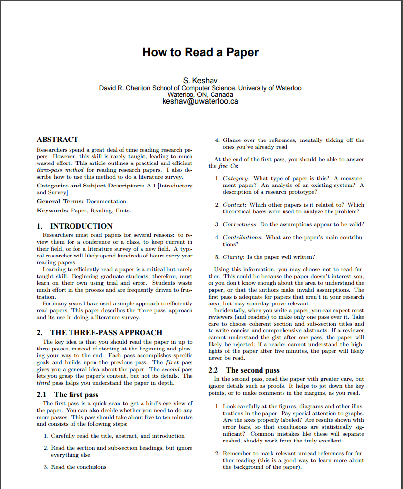
This article outlines a practical 3-pass method for reading research papers.
-
First pass: 5~10 minutes reading.
-
The following routines should be taken:
- Carefully read the title, abstract, introduction;
- Read section & sub-section headings but ignore everything else.
- Read the conclusion.
- Glance over references, ticking off the ones you have read.
-
Questions needed to be answered through this pass (“5Cs”):
-
Category: measurement paper, analysis of existing systems, or new research prototype etc.
-
Context: try to cluster within the paper the a). basic math background (Bayes formula, marginalization, SVD etc.); b). background papers (some papers which is set to be the first-reads before this paper) c). theories (some theorems provided and proved in this paper).
-
Correctness: are the assumptions made in this paper make sense to you, e.g. is the i.i.d. assumption made appropriate? Is the conditional independence assumption proper?
-
Contributions: what is the main contributions of the paper? Does that make sense to you? (Some papers will list their contributions explicitly like in the following paper. Most papers will claim their contributions in the
Introductionsection.)
-
Clarity: is this paper well-written? Some words or sentences you can use to amplify your language ability.
-
-
As the author of “How to read a paper” says, “The first pass is adequate for papers that aren’t in your research area.”
-
-
Second pass: 60 minutes reading.
-
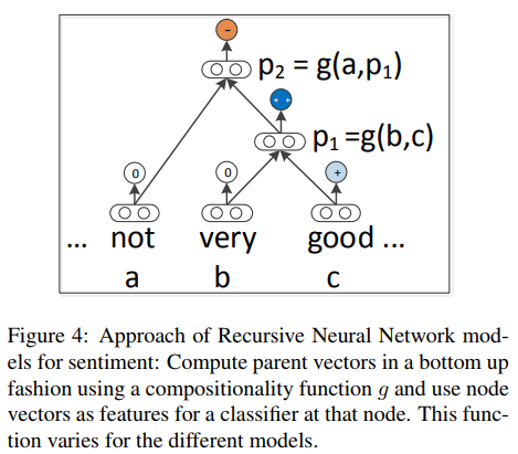
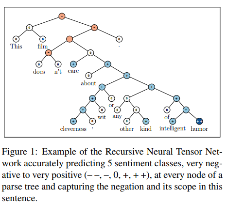
Look carefully at the figures, diagrams and other illustrations in the paper, like the following architecture for recursive neural networks for sentiment analysis and its demonstrative case example, this will make you quickly understand the overall structure of the model.
-
Look at the experiment result is also a VERY IMPORTANT part of this reading pass. Because by doing this, you can know actual experimental result and compare it with some papers you have previously read. This will ensure your belief of this paper and decide whether you should try its proposed method or not!
-
Mark relevance unread references for further reading.
-
-
Third pass: 5~6 hours reading.
- This pass is towards fully understanding of the paper. You should identify and challenge assumption in every statement made by the authors.
- The key to this pass is to attempt to virtually re-implement the paper and the experiment.